
For the proper functioning, guarantee of safety and integrity of living beings and the environment that surround them, it is essential that intelligent systems such as robots and autonomous cars, for example, are equipped with sensors of different natures. A common problem when using multiple sensors is ensuring they are all aligned and calibrated. In this project, it was proposed to test calibration methods between an RGB camera and a LiDAR using Computer Vision algorithms for the detection of a TAG (known object), taken as a calibration standard. Algorithms of 3D point clouds and RGB images were used to obtain coordinate correspondences (in both, simultaneously) in real and simulated environments.
Setup
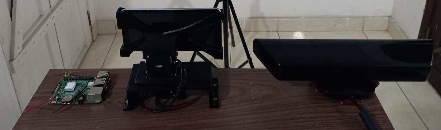
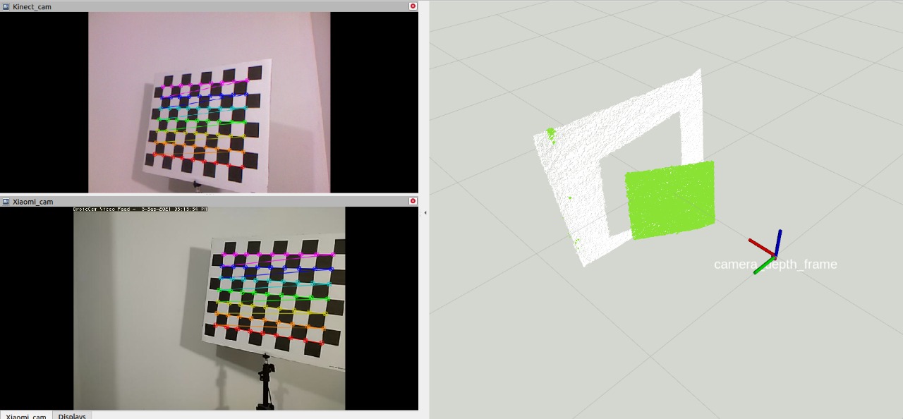
To calibrate between sensors, we first need to collect the data. As I show in the next images, this can be achieved with many sensor configurations.
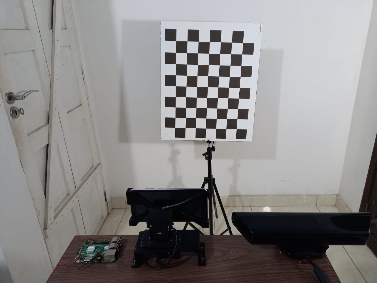 Horus setup 1
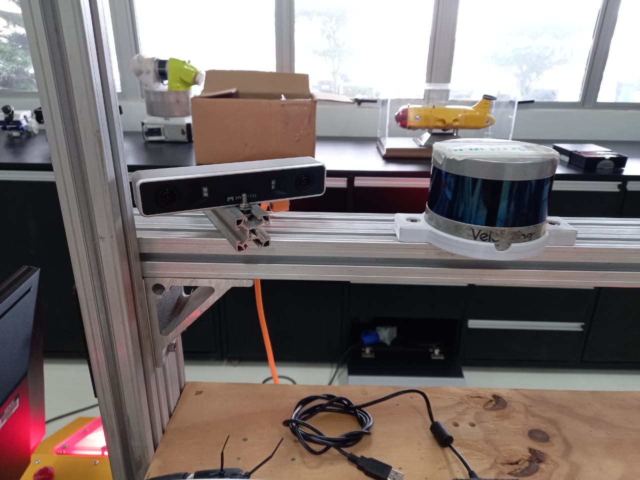 Horus setup 2
The first configuration shows us a Kinect and a regular smartphone camera. And in configuration 2 we have a Mynt Eye S 1030 sensor and a Velodyne. Both are precisely configured and have responded well to testing.
Filter
After obtaining the LiDAR data, the point clouds are pre-processed using spatial filters to delimit the field of view of interest (VoxelGrid and FrustumCulling) in order to reduce the number of analyzed points and, therefore, the time of processing. The results can be seen below, both in simulation and in a real environment.
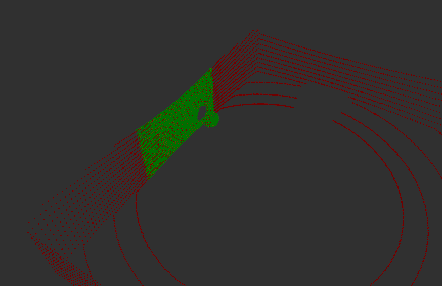 Filter in simulation. Point cloud without change (red) and pre-processed point cloud (green).
 Filter in real setup
Results with AI
Many regression methods were tested, we can use SVRPoly (Support Vector Regression, core: poly) as an example from the scikit-learn library, whose results are shown in the following figure as follows: (a) it is possible to see the arrangement of the data of test and prediction, (b) the error histogram (in pixels) between the test and predicted coordinates is represented and (c) the error in pixels between the test and predicted points is represented.
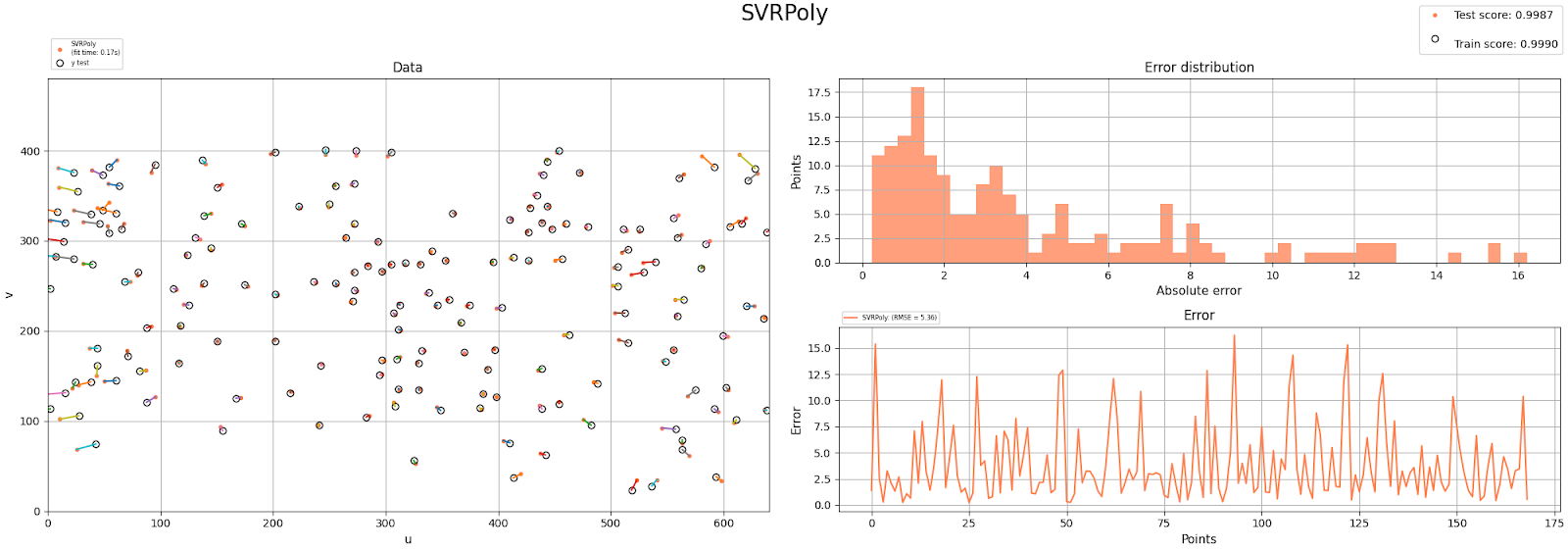 (a) Data, (b) Error distribution per histogram, (c) Error per pixel.
A total of 18 regressors from the scikit-learn library were tested and their results can be seen in the table below, which shows the mean squared deviation for the data sets and their regression scores in relation to the test set.
The qualitative analysis of the regression results can be seen below, using the SVRPoly model, by observing the colored point clouds and the arrangement of the 3d points in the image. The color associated with each three-dimensional point is the same color as the image pixel resulting from the transformation of three-dimensional coordinates.
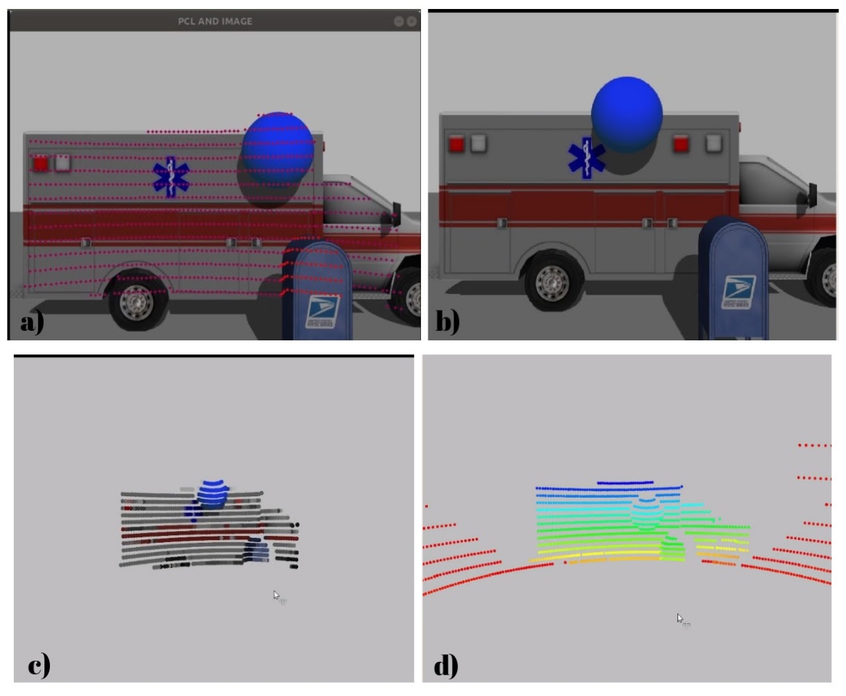 a) Camera image with inserted LiDAR points, (b) actual data acquired with the camera, (c) Post processed data by the calibration model, (d) actual data acquired with the LiDAR.
It is also possible to analyze, in the figure below, that the points projected on the camera interface contain an intensity control for the closest points (in red) and further away (in blue).
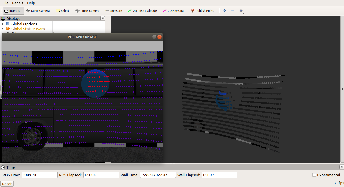 Image of camera interface with intensity points and point cloud visualization in Rviz.
For the first tests, Artificial Intelligence algorithms were used. With the evolution of the research, we chose to remove the AI part and focus on implementing a method that was just as efficient, but with a lower processing cost. The research will still generate an article, in which the method will be addressed in more depth.
3D model
A preview of the 3D model of the Horus configuration can be seen below (a test configuration as an example, could be $N$ configurations).
Development team

Project Summary
- Category: Computer Vision
- Start date: November/2019
- End date: February/2021
- Total articles produced: 1 (for more, see the publications tab)