
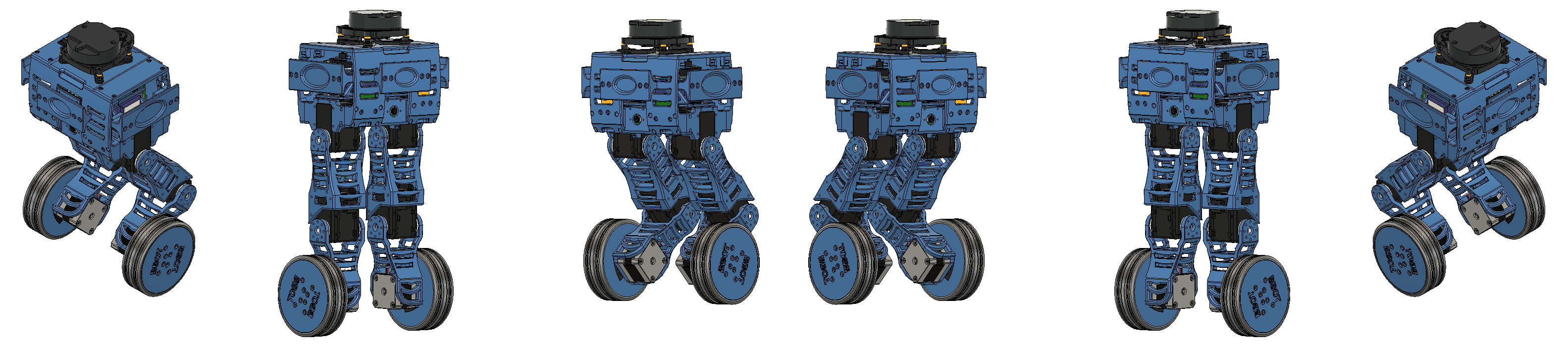
Previously
It is important that you have seen the previous post Bbot Mechanical Drawing, for a complete understanding of the project’s development.
Introduction
In step four of the Bbot construction process, we can analyze the development of its simulation made in Gazebo, using ROS Noetic.
In case you didn’t know, the Robot Operating System (ROS) is an OpenSource robotics framework with several tools implemented to facilitate the development of robotics applications. You can refer to this link for more information about ROS. For the development of Bbot, we are using the Noetic version of ROS.
System Representation and Control
Bbot, like many other high-balancing robots, can be treated as an inverted pendulum. Unlike a conventional pendulum, this system aims to balance its rod in a vertical upward position, as shown in the figure below.
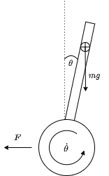 Inverted pendulum.
By letting it swing freely, the pendulum will fall until it touches the ground. However, if a force is exerted on the base of the robot, in order to move it forward or backward, a pseudo-force (which is inertia) will act on the rod in the opposite direction to the torque applied by its own weight. With the right force, we can make the pendulum swing back to an upright position. As this position is unstable, the rod will fall again and, therefore, another force must be applied.
If we can monitor the instantaneous inclination of the pendulum and, from there, calculate and exert the appropriate force for it to return to the vertical position, we will be able to keep it in balance. The following is the block diagram of the system.
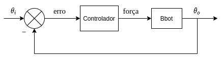 Block diagram.
This is a feedback system, where we will be sending the robot’s balance tilt as input (~ 0°) and sending the difference between this and the robot’s current tilt to the controller. This signal, called an “error”, is input from the controller, which it will use to calculate the force required to keep the Bbot in balance.
The controller will be of the PID (Proportional - Integral - Derivative) type. This type of controller is one of the most widely used in control systems. It can be described by the following equation:
 PID Equation.
As we can see, it has 3 configuration parameters: Kp, Ki and Kd. Each of these influences the speed of recovery from the equilibrium position, the time needed for it to stabilize in that position, and the type of transient response that the system will have to reach equilibrium. In case you want to know more about the PID controller, you can access this link.
Setting up the simulation in ROS
To be able to simulate the Bbot in ROS, we have created a URDF (Unified Robot Description Format) file, which contains all the information needed to simulate the robot in Gazebo. In this file, all the moving parts of the robot are defined, as well as the type of joints, inertial and collision parameters, in addition to the visual aspects, based on the mechanical design we made and showed in the previous post (click here to learn more).
In order to be able to send speed commands to the robot and be able to move it forward and backward, as well as rotate around its own axis, we used a differential direction controller implemented in ros_control package.
Since the Bbot has articulated legs, we also set up position controllers for each of its joints. However, for this simulation, we will not use leg control.
Until then, it would be possible to move the robot, but for it to be autonomous, some sensors are needed so that it can sense the environment around it, get a sense of its position and orientation in space, and see what is in front of it. Therefore, also in the URDF, we configured the Gazebo plugins that simulate an IMU (Inertial Mesurement Unit) sensor, to monitor the robot’s inclination as well as its speed and angular acceleration in 3 dimensions; a Lidar (Light Detection and Ranging), to identify possible obstacles and a camera, which allows us to use computer vision to give the robot more intelligence.
We then created three packages to store all this information:
- bbot_description: Contains the URDF file and the Bbot render files.
- bbot_gazebo: Contains the virtual world file and .launch files to start the simulation.
- bbot_control: Contains the configuration files of the joint controllers in addition to the control algorithm that keep the robot balanced.
With all this configured, we can already see the robot in the Gazebo and also in the Rviz.
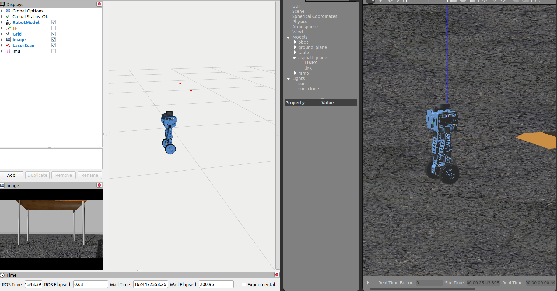 Bbot in Gazebo.
Control Algorithm
To create the robot control algorithm, we use a ROS pid, package, which implements a PID type controller that already uses the entire ROS interface as topics and parameters. This package contains a node that, after receiving a message from the topic /setpoint, is enabled, and whenever it receives a message from the topic /state, calculates the error between them, applies the PID formula, and publishes another message to the topic /control_effort. The process happens asynchronously, so it is up to the user to keep the publications in /state as constant as possible at the frequency they want. Keeping the control loop at a single frequency increases controller accuracy and improves results. In the case of Bbot, the control loop runs at 100 Hz, which is the frequency of acquisition of the tilt information, provided by the IMU.
Since the controller algorithm is already ready, we created a node that only redirects the necessary information shared by the ROS interface to the right topics with the proper message format. If you’re hearing these terms referring to ROS for the first time, it’s worth taking a look at this tutorial: link.
A graphical representation of the processes that occur in ROS can be seen in the figure below.
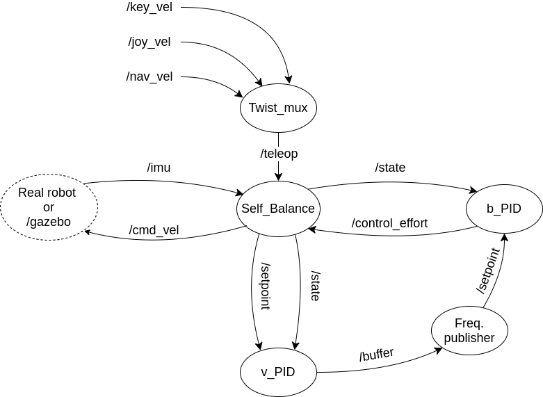 Rosnode Diagram.
In this image, there are two PID controllers. The /balancing_pid controller calculates the control effort needed to keep the robot balanced at a specific angle, while the /velocity_pid controller determines what this angle should be, based on the velocity commands the robot receives from the user or, eventually, from a trajectory planner.
The /freq_pub node serves to reduce the publication frequency on the /setpoint topic of the /balancing_pid controller, in order to decrease noise in the control. Since these messages change the balance angle and the robot needs time to stabilize, we noticed in the simulation that making changes every 0.01 seconds generated a lot of noise in the controller.
A block diagram representation of the same system can be seen below.
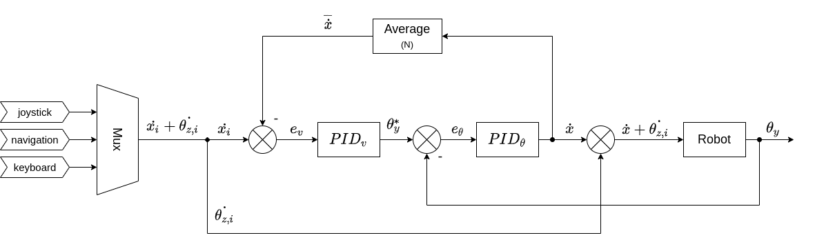 Control Diagram.
It can be noted that the data fed back to the /velocity_pid controller is not the robot’s most recent velocity command, but rather the average of the last N commands. We used N = 100. This approach also helps to reduce noise in the controller, since velocity commands can vary rapidly, but their average provides more stable and easier-to-control information.
Simulation Results
After several days of tuning the controller parameters and improving the system, we managed to make Bbot balance itself and teleoperate it.
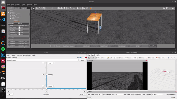 Bbot teleoperation.
We also tested its response to external forces:
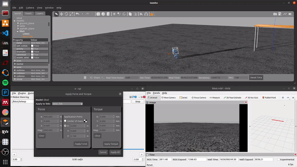 External forces test.
In the fourth stage of the project, we presented the development of the control system and teleoperation of Bbot.
In the next stages, we will cover the printing and assembly of the robot, as well as system tests with the real robot.
Author

References
- The original post was published on braziliansinrobotics, which is a project of the Brazilian Institute of Robotics (BIR). The website is no longer available, so I am reposting it here.
This is an automatically translated version of the original post from the site ‘brazilians in robotics’ (no longer available).