
When we imagine robots interacting with people or performing tasks previously done by humans, we always think about the effectiveness and precision they can achieve. Unlike a person, a robot can be designed to handle various levels of external disturbances so that these do not impact the final outcome of its mission. For this, control theory is fundamental, as it provides several tools that allow engineers to analyze robotic systems and design controllers so that they perform tasks with high precision and reliability.
Nowadays, when we think about analyzing control systems, we remember software like MATLAB or Octave, which have many tools for system analysis and controller design. However, there are now Python libraries that provide some of these tools, and together with the wide range of other applications implemented for the language, they can make system analysis extremely rich and accessible, since it is Open Source.
In this article, we will show how we used Python to analyze the control systems of Bbot (a self-balancing robot) and design an LQR (Linear Quadratic Regulator) controller using some essential packages:
If you landed here and don’t know what Bbot is, don’t worry, there will be a brief description below, but if you want to know more about the project you can access the Bbot and follow all our posts about its development.
A tip: if you want to follow along with this article, use the Google Colab file we made, so you can run the code snippets and visualize the plots and sympy equations in LaTeX.
Generating the Mathematical Model
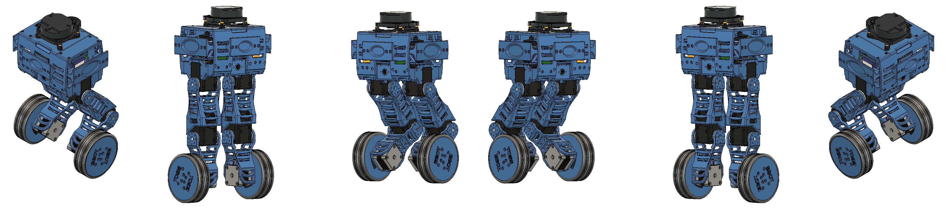
Bbot is a self-balancing robot that balances on two wheels and can thus navigate indoor environments. Its operating principle is very similar to that of an inverted pendulum: it needs a controller to keep it always upright and allow it to move in two dimensions in space.
 Bbot.
Bbot.
As seen in the image above, Bbot has two legs that allow it to squat and stand up, so it is not exactly the same as an inverted pendulum. However, since these joints should remain static most of the time, we assume sufficient similarity so that we could base ourselves on ready-made models of this type of robot, instead of creating a more specific model for Bbot (maybe for future work…). In our analysis, we based it on the model used by Kollarčík in [1], which was generated by Kim and Kwon in [2]. The analysis process shown will also follow the control design presented in [1].
We started the analysis by transcribing the model matrices shown in [2] into Python. Since this model depends on several physical parameters of the robot such as mass, moments of inertia, wheel radius, etc., we used symbolic math from sympy for this. The code is as shown below.
1
2
3
4
5
6
7
8
9
10
11
12
13
14
15
16
17
18
19
20
21
22
23
24
25
26
27
28
29
30
31
32
33
34
35
36
37
38
39
40
41
42
43
44
45
46
47
48
49
50
51
52
53
54
55
56
57
58
59
60
61
62
63
64
import numpy as np
from sympy import *
import matplotlib.pyplot as plt

#--- Model Parameters ---
d       = symbols('d',    real=True, positive=True)         # Distance between wheels
visc    = symbols('c_alpha',real=True)                      # Viscous, damping constant
l       = symbols('l',    real=True, positive=True)         # Height of the COM
r       = symbols('r',    real=True, positive=True)         # Radius of the wheel
Mp      = symbols('M_p',  real=True, positive=True)         # Mass of the pendulum without the wheels
Mw      = symbols('M_w',  real=True, positive=True)         # Mass of each wheel
Iw_c    = symbols('I_wc',  real=True)                       # MOI wheel center
Iw_r    = symbols('I_wr',  real=True)                       # MOI wheel radial
Ip_x    = symbols('I_px',  real=True)                       # MOI pendulum x
Ip_y    = symbols('I_py',  real=True)                       # MOI pendulum y
Ip_z    = symbols('I_pz',  real=True)                       # MOI pendulum z

#--- Constants & Aux. variables ---
g = symbols('g', constant=True)                             # Gravity acceleration
t = symbols('t', real=True)                                 # Time

#--- State Variables ---
x           = symbols('x',  real=True)                      # Linear pos
pitch       = symbols('theta',  real=True)                  # Pitch angle
yaw         = symbols('psi',  real=True)                    # Yaw angle
x_vel       = Derivative(x,t)                               # Linear vel
pitch_vel   = Derivative(pitch,t)                           # Pitch vel
yaw_vel     = Derivative(yaw,t)                             # Yaw vel
x_acc       = Derivative(x_vel,t)                           # Linear acc
pitch_acc   = Derivative(pitch_vel,t)                       # Pitch acc
yaw_acc     = Derivative(yaw_vel,t)                         # Yaw acc

#--- Inputs ---
Tl = symbols('T_L', real=True)                              # Torque of the left wheel
Tr = symbols('T_R', real=True)                              # Torque of the right wheel

#*--- Matrices for the 3 states model
M = Matrix([[Mp+2*Mw+2*Iw_c/r**2, Mp*l*cos(pitch) ,                                                                     0],
            [ Mp*l*cos(pitch)   , Ip_y+Mp*l**2    ,                                                                     0],
            [0                  ,                0, Ip_z+2*Iw_r+(Mw+Iw_c/r**2)*d**2/2-(Ip_z-Ip_x-Mp*l**2)*sin(pitch)**2  ]])

C = Matrix([[                      0, -Mp*l*pitch_vel*sin(pitch),                          -Mp*l*yaw_vel*sin(pitch)],
            [                      0,                          0, (Ip_z-Ip_x-Mp*l**2)*yaw_vel*sin(pitch)*cos(pitch)],
            [Mp*l*yaw_vel*sin(pitch), -(Ip_z-Ip_x-Mp*l**2)*yaw_vel*sin(pitch)*cos(pitch), -(Ip_z-Ip_x-Mp*l**2)*pitch_vel*sin(pitch)*cos(pitch)]])

D = Matrix([[2*visc/r**2, -2*visc/r, 0],
            [-2*visc/r, 2*visc, 0],
            [0, 0, (d**2/(2*r**2))*visc]])

B = Matrix([[     1/r,     1/r],
            [      -1,      -1],
            [-d/(2*r), d/(2*r)]])

G = Matrix([[0],[-Mp*l*g*sin(pitch)], [0]])

q = Matrix([[x],[pitch],[yaw]])

q_diff = Matrix([[x_vel],[pitch_vel],[yaw_vel]])

q_2diff = Matrix([[x_acc],[pitch_acc],[yaw_acc]])

u = Matrix([[Tl],[Tr]])

M_inv = M.inv()
In the section above, we defined all the symbols we will use, created the system matrices using the Matrix class from sympy, and, as needed, computed the inverse of M by calling one of the class methods. The advantage of working with symbolic math is that all calculations are in terms of symbols, so there are no approximation or truncation errors as with floating-point operations.
Following the referenced articles, we generate a system vector with three differential equations and display the result.
1
2
3
expr_model = M_inv*((B*u-G)-(C+D)*q_diff)
eqts_model = Eq(q_2diff,expr_model)
eqts_model # Displaying the variable alone in Jupyter shows its output.
As seen in the output, this model is a system of 3 nonlinear differential equations modeling the linear, yaw (rotation around the z-axis), and pitch (rotation around the y-axis) velocities. From these equations, we can generate a state-space model of the system with these variables as states. However, for this robot, we can expand the model to control other information, such as the linear, pitch, and yaw positions. The pitch position is especially important, as we not only want the robot not to fall (pitch velocity = 0), but also to keep it upright (pitch position = 0). Thus, we can add these 3 states to the model as shown in the snippet below. To make the analysis easier later, we replace the state symbols with x1, x2, x3, x4, x5, x6 and show their correspondence with the previous symbols in the last line.
1
2
3
4
5
6
7
#* Convert real variables into state-space variables

# Build state vector
real_state_vec = q_diff.row_insert(4,q)
state_vec = Matrix(list(symbols('x1:7',real=True)))
state_eq = Eq(state_vec,real_state_vec)
state_eq
We can now include the new states in the previous system and replace their symbols with x1, x2, x3, x4, x5, x6.
1
2
3
4
5
6
7
8
9
10
11
12
13
#* Build the vector of system equations

system_equations = expr_model.row_insert(4,q_diff)

#* Substitute the real variables with the state-state model variables: x1:x6

for i in range(6):
  system_equations = system_equations.subs(real_state_vec[i],state_vec[i])

#* Show the system of equations that will be used in the state space form

eq_sys = Eq(state_diff_vec,system_equations)
eq_sys
System Linearization
Up to this point, we have a system of nonlinear differential equations containing all the information we need to control the robot. However, as mentioned, this system is nonlinear (due to all the sine and cosine terms), and to design an LQR controller, we need to linearize it. If we use the approximation that, for angles close to zero, sine and cosine are approximately equal to the angle itself and 1, respectively, we can work with a linear system, provided the robot is near the upright position (small pitch angles). Therefore, we will linearize the system around this equilibrium point, known as the fixed point. Although this fixed point is an equilibrium of the system, it is unstable, since any small deviation will cause the robot to fall.
To linearize the system, we will calculate the Jacobian matrix of the system with respect to the states and control inputs. The states were mentioned above, and our control inputs are the torques applied to each wheel. In other words, we intend to control the system by sending torque commands to the wheel motors so that the state values tend toward zero (or any other fixed point you choose, but for this system it will be zero) over time. We calculate the Jacobian matrix using sympy as shown below.
1
2
3
4
5
6

#* Calculate the jacobian for the A and B matrix of the continuos time system
Ac = system_equations.jacobian(state_vec)
Bc = system_equations.jacobian(u)
# Ac
# Bc
In the first line, we compute the Ac matrix (the A matrix of the state-space model from the continuous-time system), which is the Jacobian of the system—these are the partial derivatives of the system equations with respect to the states. The Bc matrix is the Jacobian with respect to the control inputs. You can uncomment the last lines to display the matrices in the notebook.
We now have the linearized matrices, but they are still symbolic. In the next steps, we will substitute these symbols with numerical values using the subs method from sympy, as shown below.
1
2
3
4
5
6
7
8
9
10
11
12
13
14
15
16
17
18
19
20
21
22
23
24
25
26
27
28
29
30
31
32
33
34
35
36
37
38
39
40
41
42
43
44
45
46
47
48
49

#* Evaluate Ac and Bc at the fixed points

fixed_point = [0,0,0,0,0,0] # Values for dx/dt
input_fixed_points = [0,0]

Ac_eval = Ac.subs([(state_vec[0], fixed_point[0]),
                   (state_vec[1], fixed_point[1]),
                   (state_vec[2], fixed_point[2]),
                   (state_vec[3], fixed_point[3]),
                   (state_vec[4], fixed_point[4]),
                   (state_vec[5], fixed_point[5]),
                   (Tl,input_fixed_points[0]),
                   (Tr,input_fixed_points[1])])

Bc_eval = Bc.subs([(state_vec[0], fixed_point[0]),
                   (state_vec[1], fixed_point[1]),
                   (state_vec[2], fixed_point[2]),
                   (state_vec[3], fixed_point[3]),
                   (state_vec[4], fixed_point[4]),
                   (state_vec[5], fixed_point[5]),
                   (Tl,input_fixed_points[0]),
                   (Tr,input_fixed_points[1])])


# Define the values of each Model Parameter

d_v    = (d,    0.1431)
visc_v = (visc, 0.01)
r_v    = (r,    0.05)
Mp_v   = (Mp,   2.036)
Mw_v   = (Mw,   0.268)
Iw_c_v = (Iw_c, 0.00033613)
Iw_r_v = (Iw_r, 0.00018876)
g_v    = (g,    9.81)

#-- Pose A ---
l_v    = (l,   0.1806)
Ip_x_v = (Ip_x, 0.02500992)
Ip_y_v = (Ip_y, 0.02255237)
Ip_z_v = (Ip_z, 0.00546422)

#* Plug in the Model parameters values

Ac_lin = Ac_eval.subs([d_v,visc_v,l_v,r_v,Mp_v,Mw_v,Iw_c_v,Iw_r_v,Ip_x_v,Ip_y_v,Ip_z_v,g_v])
Bc_lin = Bc_eval.subs([d_v,visc_v,l_v,r_v,Mp_v,Mw_v,Iw_c_v,Iw_r_v,Ip_x_v,Ip_y_v,Ip_z_v,g_v])

Ac_np = np.array(Ac_lin) # Converts it into a numpy array
Bc_np = np.array(Bc_lin) # Converts it into a numpy array
To substitute the value of several symbols at once, we must pass a list of tuples containing the symbol variable and its value. First, we substitute the fixed point values, which are 0 for all variables. Then, we create tuples for each symbol related to a model parameter and the corresponding value from the Bbot’s 3D model. These values were calculated using Oneshape. Because Bbot has legs that modify some model parameters, we calculated the values for 3 different poses, as shown in the images below (A, B, and C, from left to right). Finally, we generate a numpy.array() from these matrices.
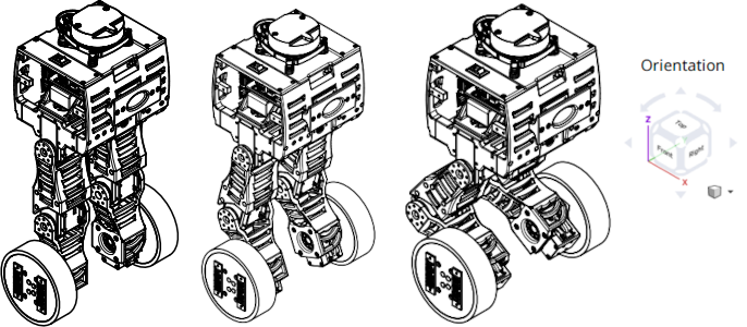 Leg components in exploded view.
System Discretization
The model we based our work on considers a continuous-time system, but we intend to generate controllers that can be implemented on a microcontroller, which operates in discrete time. Therefore, we must discretize the system. This is where the control library becomes very helpful. We can create a state-space system with the matrices we calculated and discretize the system in just two lines.
1
2
3
4
5
6
7
8
import control

Ts = 0.01 # Sampling period. Fs = 100 hz

sysc = control.ss(Ac_np,Bc_np,np.eye(6),np.zeros((6,2)))
sysd = control.c2d(sysc,Ts,method='zoh')
Ad = sysd.A
Bd = sysd.B
At the end, we store the discretized system matrices in the variables Ad and Bd. The discretization method used was zero-order hold and the sampling period was 0.01 seconds, equivalent to a sampling frequency of 100 Hz. This value is completely arbitrary and is used as a starting point for the simulation. In the future, considering the real dynamics of the robot’s motors (not covered in this article), we may adjust this period to better match the system’s dynamics. The sampling period defines the frequency of the control loop that will be implemented on the robot. In this case, our controller should send control efforts to the system at a frequency of 100 Hz.
As shown in the referenced articles, this robot does not need to control the linear and yaw positions to balance itself. Therefore, we can reduce the system to 4 states: linear velocity, pitch velocity, yaw velocity, and pitch angle. This is quite simple to do—just remove the rows of the Ad and Bd matrices corresponding to those two states. In the end, we obtain the 4x4 matrix Ar and the 4x2 matrix Br.
1
2
Ar = np.vstack(( np.hstack((Ad[0:3,0:3], Ad[0:3,4].reshape(3,1))) , np.hstack((Ad[4,0:3], Ad[4,4])) ))
Br = np.vstack(( Bd[0:3,:], Bd[4,:] ))
Adding Integral Action to the System
With the matrices Ar and Br, we can design a controller, implement it on a microcontroller, and the robot will be able to balance itself. However, Bbot is a mobile robot and should be able to receive linear and yaw velocity commands and follow these references. This allows for teleoperation or even the implementation of autonomous navigation algorithms. To achieve this, we need to ensure that the controller can receive a reference value and control the system to track it. For example, if we command “move forward at 0.3 m/s” or “turn left at 0.15 rad/s”, the controller should be able to keep the robot balanced while moving at the desired speed.
To do this, we must compute the error (the difference) between the robot’s current velocity and the reference, and feed the integral of this error to the controller. The integral action ensures that this error tends to zero, meaning the actual velocity matches the reference.
We create an augmented model of the system by including the integral of the linear and yaw velocity errors as states. The system matrices are modified as shown below.
1
2
3
4
5
6
L_aug = np.hstack((np.array([[-1,0,0,0],
                             [0,0,-1,0]]), np.eye(2) ))
Upper_aug = np.hstack((Ar, np.zeros((4,2))))
A_aug = np.vstack((Upper_aug, L_aug))

B_aug = np.vstack((Br,np.zeros((2,2))))
Control System
With the augmented system matrices A and B in hand, we proceed with system analysis and controller design. The first step is to check if this system is controllable, that is, to verify whether it is possible to drive the system states to the fixed point around which we linearized, using only the wheel torques as control inputs. We will also test if the system is observable. Control systems can have dozens of states, but not all of them can be measured by sensors. Therefore, by indicating only the states we can measure (these are the outputs of our system), we can test if the system is still observable. If it is, it is possible to design an estimator (such as a Kalman filter) that, using only the measured state data, can estimate the values of the other states and provide this information to the controller. In the case of Bbot, we have wheel encoders, which allow us to calculate the robot’s linear velocity knowing the wheel radius, and an IMU, which provides position, acceleration, and angular velocity on all three spatial axes. Therefore, we know we can measure all states, but we perform the test for completeness of the analysis.
In the code snippet below, we use the control.ctrb and control.obsv functions, which return the controllability and observability matrices of the system. If the rank of these matrices is equal to the number of system states, the system is controllable and observable.
1
2
3
4
5
6
7
8
9
10
11
12
13
#* Controllability and Observability for the augmented model

C_ss_aug = np.diag([1,1,1,1,1,1])
D_ss_aug = np.zeros((6,2))

ctrb_m = control.ctrb(A_aug,B_aug)
rank_ctrb = np.linalg.matrix_rank(ctrb_m) # If result is 6, the system is controllable

obs_m = control.obsv(A_aug,C_ss_aug)
rank_obs = np.linalg.matrix_rank(obs_m) # If result is 6, the system is controllable

print(rank_ctrb)    # 6 means Controllable
print(rank_obs)     # 6 means Observable
We can also evaluate the poles of the system to confirm our intuition that the system is unstable.
1
2
sys_aug = control.ss(A_aug, B_aug, C_ss_aug, D_ss_aug)
abs(sys_aug.pole())
Since our system is discrete, we analyze stability according to Z-transform theory. By examining the system poles, we can see that there are poles with modulus greater than or equal to 1.0, which means the system is unstable.
Running the code, we see that the rank of both matrices is indeed 6, so we can design an LQR controller for the system, and since we have all the measurements, we do not need to design an estimator. To design the controller, we need the cost matrices Q and R. These matrices contain cost values defined by the designer, indicating their performance priorities for each state (Q matrix) and the cost of the energy that can be demanded from the motors (R matrix). The control library provides a control.lqr() function that, given the system matrices and the Q and R matrices, returns the controller gain matrix K. The function also returns the solution to the Riccati equation (required for calculating K) and the poles of the controlled system. However, this function is intended for continuous-time systems. As of the date of this article, there is no discrete-time version in the library, but a user has provided a function and shared the code in an issue on the python-control repository. The usage of the function follows the same logic. Below is the function and the code snippet where we calculate the K matrix and the poles of the controlled system, and we see that all of them have modulus less than 1.0.
1
2
3
4
5
6
7
8
9
10
11
12
13
14
15
16
17
18
19
20
21
22
23
24
25
26
27
28
29
30
31
32
33
34
35
36
37
38
39
40
41
42
def dlqr_calculate(G, H, Q, R, returnPE=False):
  '''
  Discrete-time Linear Quadratic Regulator calculation.
  State-feedback control  u[k] = -K*x[k]

  How to apply the function:
      K = dlqr_calculate(G,H,Q,R)
      K, P, E = dlqr_calculate(G,H,Q,R, return_solution_eigs=True)

  Inputs:
    G, H, Q, R  -> all numpy arrays  (simple float number not allowed)
    returnPE: define as True to return Ricatti solution and final eigenvalues

  Returns:
    K: state feedback gain
    P: Ricatti equation solution
    E: eigenvalues of (G-HK)  (closed loop z-domain poles)
  '''
  from scipy.linalg import solve_discrete_are, inv, eig
  P = solve_discrete_are(G, H, Q, R)  #Solução Ricatti
  K = inv(H.T@P@H + R)@H.T@P@G    #K = (B^T P B + R)^-1 B^T P A

  if returnPE == False:   return K

  from numpy.linalg import eigvals
  eigs = np.array([eigvals(G-H@K)]).T
  return K, P, eigs

Q_lqr_aug = np.diag([1 /(0.5**2),
                     100 /(0.1**1),
                     1 /(1**1),
                     1 /(0.14**2),
                     2 /(1**2),
                     2 /(2**2)])

R_lqr_aug = np.diag([1e2 /(0.5**2),
                     1e2 /(0.5**2)])

K_dlqr_aug, S_dlqr_aug, E_dlqr_aug = dlqr_calculate(A_aug,B_aug,Q_lqr_aug,R_lqr_aug,True)

# Matrix(K_dlqr_aug)
# Matrix(abs(E_dlqr_aug).reshape(1,6)) # If all are below 1, the system is stable
System Simulation
We now have the differential equations of our system and the controller. Next, we need to simulate our nonlinear system and check if this controller can stabilize it. To simulate the system, we will use a differential equation solver provided by the scipy package. We will use the vector of differential equations we created at the beginning (with only the 4 states we selected) to create a function that, given the current state values, calculates the derivatives defined on the left side of the equation. scipy will use this to solve the system.
Below, we create another vector with the robot’s parameter values already substituted. We define the initial conditions for each state, the inputs, the initial time, and the reference values for linear and yaw velocities. Using the sympy.lambdify function, we can turn a symbolic sympy expression into a Python lambda function, whose parameters will be time, the state vector, and the input vector. By uncommenting the last line, we can evaluate the system for the defined initial values.
1
2
3
4
5
6
7
8
9
10
11
12
13
14
15
16
#* Apply model parameters to the system equations

sys2sim = system_equations.subs([d_v,visc_v,l_v,r_v,Mp_v,Mw_v,Iw_c_v,Iw_r_v,Ip_x_v,Ip_y_v,Ip_z_v,g_v])
sys2sim.row_del(3)
sys2sim.row_del(4)

state_initial_conditions = [0,0,0,0]
initial_inputs = [0,0]
x_yaw_refs = np.array([0.2, 1]) # 0.2 m/s and 1 rad/s
t0 = 0

#* Create lambda functions of the system
reduced_state_vec = Matrix(list(symbols('x1:4, x5',real=True)))
func = lambdify([t, reduced_state_vec, u],sys2sim,'numpy')

# func(0,state_initial_conditions, initial_inputs) # Test the lambda function
Using the integrate.ode class from scipy, we simulate the system for up to 10 seconds with a time step of 0.01 seconds. We also include white noise and apply a torque pulse of 0.3 Nm to the wheels from 6 to 6.3 seconds. Throughout the simulation, we store the values of the states, inputs, and time in a numpy.array so we can plot the results later. At the end of the simulation, we calculate the integral of the linear velocity curve to plot the robot’s position over time.
1
2
3
4
5
6
7
8
9
10
11
12
13
14
15
16
17
18
19
20
21
22
23
24
25
26
27
28
29
30
31
32
33
34
35
36
37
38
39
40
41
42
43
44
45
46
47
48
49
50
51
52
53
54
55
56
from scipy import integrate

simulator = integrate.ode(func)                                     # Ode class object used for simulation
simulator.set_initial_value(state_initial_conditions, t0)           # Set initial conditions of the system
simulator.set_integrator('vode')
simulator.set_f_params(initial_inputs)                              # Set the initial inputs (wheel torques) values in the system
# simulator.set_jac_params(initial_inputs)                            # Set the initial inputs (wheel torques) values in the jacobian

t1 = 10                                                           # Max. time for simulation
dt = 0.01                                                          # Simulation time step
controller_time = 0                                                # Initial controller time (-1 means: "provide a control effort based on the initial states")
controller_calls = 0                                                # Counts how many times the controller was called (just debug)

history = np.array([state_initial_conditions]).reshape(4,1)
# time_history = [t0]
time_history = np.arange(start=0,stop=t1+2*dt,step=dt)
input_history = np.array(initial_inputs).reshape(2,1)

Kp = K_dlqr_aug[:,0:4]
Ki = K_dlqr_aug[:,4:]

x_error = 0
yaw_error = 0
x_yaw_refs = np.array([0.2, 1])

mag_NOISE_y = 1e-3 # Magnitude of white noise

while simulator.successful() and simulator.t <= t1:                 # Simulation main loop
    history = np.hstack((history,np.array([simulator.integrate(simulator.t+dt)]).reshape(4,1) + np.random.rand(4,1)*mag_NOISE_y))        # Simulate one time step and save in history
    # time_history.append(simulator.t+dt)

    if simulator.t > 3:                         # Apply a reference change for X and Yaw vel
        x_yaw_refs = np.array([-0.3, 0])

    if simulator.t > 6 and simulator.t < 6.3: uIMPULSE = 0.3                      # Apply a torque pulse as external disturbance from time 3 - 4
    # elif simulator.t in time_history[int(3/dt):int(4/dt)]: uIMPULSE = -0.3
    else: uIMPULSE = 0.0
    controller_time += 1

    x_error += x_yaw_refs[0] - history[0,-1]
    yaw_error += x_yaw_refs[1] - history[2,-1]
    error_matrix = np.array([x_error,yaw_error]).reshape(2,1)

    regulatory_part = -Kp@history[:,-1]
    integral_part = -Ki@error_matrix

    # Call the controller
    input_history = np.hstack((input_history,regulatory_part.reshape(2,1) +
                               integral_part.reshape(2,1) +
                               uIMPULSE))

    simulator.set_f_params(input_history[:,-1])       # Update the controller values in the systems equations

print(simulator.get_return_code())

x_pos = integrate.cumtrapz(y = history[0,:],x = time_history,initial=0) # Integrate the Velocity values to get position information
Next, we plot the results using matplotlib.
1
2
3
4
5
6
7
8
9
10
11
12
13
14
15
16
17
18
19
20
21
22
23
24
25
26
27
28
29
30
31
32
33
34
35
36
37
38
39
40
41
42
43
fig1 = plt.figure()
plt.plot(time_history,history[0,:])
plt.title("Linear vel")
plt.xlabel("time (s)")
plt.ylabel("m/s")
plt.grid()

fig2 = plt.figure()
plt.plot(time_history,history[1,:])
plt.title("Pitch vel")
plt.xlabel("time (s)")
plt.ylabel("rad/s")
plt.grid()

fig3 = plt.figure()
plt.plot(time_history,history[2,:])
plt.title("Yaw vel")
plt.xlabel("time (s)")
plt.ylabel("rad/s ")
plt.grid()

fig4 = plt.figure()
plt.plot(time_history,history[3,:])
plt.title("Pitch")
plt.xlabel("time (s)")
plt.ylabel("rad")
plt.grid()

fig5 = plt.figure()
plt.plot(time_history,input_history[0,:], label='Left Torque')
plt.plot(time_history,input_history[1,:], label='Right Torque')
plt.title("Wheel Torques")
plt.legend()
plt.xlabel("time (s)")
plt.ylabel("N.m")
plt.grid()

fig7 = plt.figure()
plt.plot(time_history,x_pos)
plt.title("X positions")
plt.xlabel("time (s)")
plt.ylabel("m")
plt.grid()
From the plots, we can analyze the system’s performance over the entire simulation period. By examining the torque and linear velocity data, for example, we can assess whether these values are within the operating range of the robot’s actuators. If they are not, we can adjust the controller cost matrices or simulate smaller disturbances to explore the robot’s operational limits.
Finally, to provide a more visual analysis of the simulation, we also created an animation using the matplotlib library.
1
2
3
4
5
6
7
8
9
10
11
12
13
14
15
16
17
18
19
20
21
22
23
24
25
26
27
28
29
30
31
32
33
34
35
36
37
38
39
40
41
42
43
44
45
46
47
48
49
50
51
52
53
54
55
56
57
58
59
60
61
62
63
#Generates an animation using Matplotlib

from matplotlib.patches import Circle
from matplotlib.animation import FuncAnimation

xlim = (-1.5,1.5)
ylim = (-0.1,1.0)

fig = plt.figure(figsize=(8.3333, 7.25), dpi=72) #figsize=(8.3333, 7.25), dpi=72
ax = fig.add_subplot(111,xlim=xlim,ylim=ylim)
ax.set_aspect('equal')
ax.grid(alpha = 0.3)

height = 0.354

ax.plot([xlim[0],xlim[1]],[0,0],'-k')         # Ground

pend_rod, = ax.plot([x_pos[0], x_pos[0]+height*np.math.sin(history[3,0])],[r_v[1],r_v[1] + height*np.math.cos(history[3,0])], 'r', lw=3)
pend_wheel = ax.add_patch(Circle((x_pos[0],r_v[1]), r_v[1], fc='b', zorder=3))
time_template = 'time = %.3fs'
x_ref_template = 'X_vel input = %.1f m/s'
yaw_ref_template = 'Yaw_vel input = %.1f rad/s'

x_curr_template = 'Current X_vel = %.3f m/s'
yaw_curr_template = 'Current Yaw_vel = %.3f rad/s'


time_text = ax.text(0.02, 0.9, '', transform=ax.transAxes)
x_ref_text = ax.text(0.02, 0.8, '', transform=ax.transAxes)
yaw_ref_text = ax.text(0.02, 0.7, '', transform=ax.transAxes)
x_curr_text = ax.text(0.35, 0.8, '', transform=ax.transAxes)
yaw_curr_text = ax.text(0.35, 0.7, '', transform=ax.transAxes)

def init_anim():
  pend_rod, = ax.plot([x_pos[0], x_pos[0]+height*np.math.sin(history[3,0])],[r_v[1],r_v[1] + height*np.math.cos(history[3,0])], 'r', lw=3)
  pend_wheel = ax.add_patch(Circle((x_pos[0],r_v[1]), r_v[1], fc='b', zorder=3))
  time_text.set_text('')
  x_ref_text.set_text('')
  yaw_ref_text.set_text('')
  x_curr_text.set_text('')
  yaw_curr_text.set_text('')
  return pend_rod, pend_wheel, time_text, x_ref_text, yaw_ref_text, x_curr_text, yaw_curr_text

def animate(i):
  xaxis = [x_pos[i], x_pos[i] + height*np.math.sin(history[3,i])]
  yaxis = [r_v[1], r_v[1] + height*np.math.cos(history[3,i])]
  pend_rod.set_data(xaxis,yaxis)
  pend_wheel.set_center((x_pos[i],r_v[1]))

  time_text.set_text(time_template % (time_history[i]))
  x_curr_text.set_text(x_curr_template % (history[0,i]))
  yaw_curr_text.set_text(yaw_curr_template % (history[2,i]))

  if time_history[i] > 3:
    x_ref_text.set_text(x_ref_template % (-0.3))
    yaw_ref_text.set_text(yaw_ref_template % (0.0))
  else:
    x_ref_text.set_text(x_ref_template % (0.2))
    yaw_ref_text.set_text(yaw_ref_template % (1.0))

  return pend_rod, pend_wheel, time_text, x_ref_text, yaw_ref_text

anim = FuncAnimation(fig, animate,frames=len(time_history),interval=10,blit=True)
To visualize the result, we save the animation as a .gif file.
1
anim.save("Gifs/disturbance3.gif", fps=36) #Generates a .gif for the animation
Example of generated gif:
 Model gif.
Conclusion
As shown in the gif above (and hopefully you also followed our development through the Google Colab file), we were able to use a mathematical model of a self-balancing robot to design an LQR controller that allows the robot to balance itself and, in addition, follow linear and angular (Yaw) velocity commands based on a reference provided by us. This forms the foundation upon which we can extend Bbot’s functionalities, such as adding control to the leg joints to make it robust to certain obstacles in the environment or implementing autonomous navigation algorithms, for example.
However, before doing anything else, Bbot needs to balance itself, and using an LQR controller offers great reliability for this, as it is quite robust to certain model imperfections and allows for a wide operating range. This can be seen by changing the parameters of the Q and R matrices and observing the system’s performance changes. By doing this (and I recommend you try it), you will notice that it is possible to balance the system in various ways, prioritizing the stability of certain states or allowing more or less torque to be demanded from the wheels to suit a specific actuator. Increasing the cost of the linear velocity error state (by increasing the corresponding value in the Q matrix), for example, will make the robot reach the reference more quickly, but at the same time, it will require motors with a faster response. However, the system may not have such fast motors or may have motors with low torque, so you can prioritize a lower linear velocity and less torque on the motors (by increasing the corresponding value in the R matrix), at the cost of a system with a slower response to commands and less ability to handle external disturbances, but still able to balance itself. This depends on the actual system to be built, and it is great that this is the case, as it shows that it is possible to use the same modeling and controller for various applications.
Another focus of this post was the exclusive use of the Python language. As seen, we used several tools implemented for it, but there are many more, showing that Python is already a great open-source tool for analyzing and modeling control systems. If you want to know more about the packages we used, just access the online documentation at the links below.
And if you want to know more about the Bbot project, you can visit our official page.
Author

References
- Adam Kollarčík; Modeling and Control of Two-Legged Wheeled Robot; Master’s thesis, CZECH TECHNICAL UNIVERSITY IN PRAGUE. 2021.
- Kim, Sangtae; Kwon, Sang Joo; “Dynamic modeling of a two-wheeled inverted pendulum balancing mobile robot”, p. 926-933 . In: International Journal of Control, Automation and Systems. 2015.
- The original post was published on braziliansinrobotics, which is a project of the Brazilian Institute of Robotics (BIR). The website is no longer available, so I am reposting it here.
This is an automatically translated version of the original post from the site ‘brazilians in robotics’ (no longer available).