
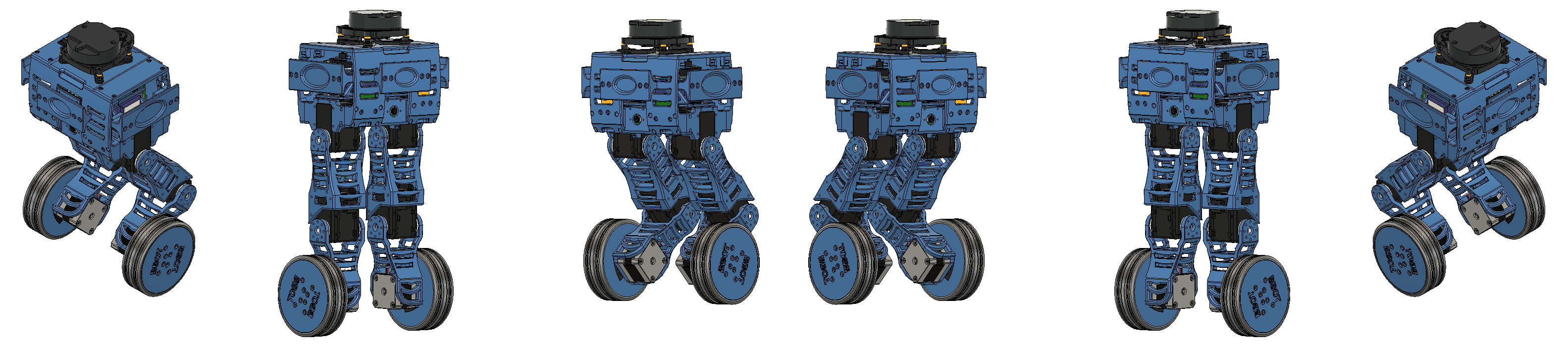
Control systems can be represented by a set of mathematical equations known as a mathematical model. These models are useful for the analysis and design of control systems. As described in the previous post, Bbot Real Tests, the PID controller was not able to stabilize the robot. Therefore, we decided to conduct a more in-depth study of the robot’s mathematical model and control. A search for articles and similar works on self-balancing robots was carried out, and in the end, two articles stood out and formed the basis for our development: Modeling and Control of Two-Legged Wheeled Robot by Adam Kollarčík and Dynamic modeling of a two-wheeled inverted pendulum balancing mobile robot by Sangtae Kim and Sang Joo Kwon.
Model
We know that models for most pendulum-like systems are well established, and our model (Bbot) is no exception. Therefore, as referenced, we used a model from the previous articles. The state-space model is as follows:
$$ \begin{bmatrix}\ddot{x}\\ \ddot{φ}\\ \ddot{ψ} \end{bmatrix} = \begin{bmatrix}m_{11} & m_{12} & 0\\ m_{21} & m_{22} & 0\\ 0 & 0 & m_{33} \end{bmatrix}^{-1} \begin{pmatrix} \begin{bmatrix} \frac{1}{r_0}(u_{0R} + u_{0L}) \\ m_plg\sin φ - u_{0R} - u_{0L} \\ \frac{w}{2}(u_{0R} - u_{0L}) \end{bmatrix} - \begin{bmatrix} \frac{2b}{r_0^2} & d_{12} & d_{13}\\ \frac{-2b}{r_0} & 2b & d_{23}\\ d_{31} & d_{32} & d_{33} \end{bmatrix} \begin{bmatrix}\dot{x}\\ \dot{φ}\\ \dot{ψ} \end{bmatrix} \end{pmatrix} $$
Where:
$$ m_{11} = m_p + 2m_0 + 2\frac{I_0}{r_0^2}, m_{12} = m_{21} = m_pl\cos φ, m_{22} = I_{py} + m_pl^2, $$ $$ m_{33} = I_{pz} + 2I_{0xy} + (m_0 + \frac{I_0}{r_0^2})\frac{w^2}{2} - (I_{pz} - I_{px} - m_pl^2) \sin^2 φ, $$ $$ d_{12} = -m_pl\dot{φ}\sin φ - \frac{2b}{r_0}, d_{13} = m_pl\dot{ψ}\sin φ, d_{23} = (I_{pz} - I_{px} - m_pl^2)\dot{ψ}\sin φ\cos φ, $$ $$ d_{31} = m_pl\dot{ψ}\sin φ, d_{32} = -d_{23}, d_{33} = -(I_{pz} - I_{px} - m_pl^2)\dot{φ}\sin φ \cos φ + \frac{w^2}{2r_0^2}b $$
We have parameters such as inertia, mass, distance between wheels, wheel torque, gravity, and friction coefficient. It is worth mentioning that $x$ is the distance traveled by the pendulum, $φ$ is the pitch angle, and $ψ$ is the yaw angle.
We decided to simplify the model by using static joints. The movement of the upper joints will be implemented in the next stages. All parameter values mentioned were taken from the technical drawing made in the Onshape software.
The next step in development is the linearization of the system, obtaining the matrices $Ac$ and $Bc$. These matrices are found from the Jacobian with respect to the state vector and the wheel torque. These matrices are evaluated at a fixed point, which in our case, were all at 0.
The system is then discretized, obtaining the matrices $Ad$ and $Bd$, using the zero-order hold method with a frequency set to 25 Hz.
Control
In many articles, we came across the LQR controller and observed its good performance in such systems. Since we did not have a very efficient implementation with PID, we chose to implement a similar method, but with a difference: using LQR on the discretized system, so we used the Discrete-time Linear Quadratic Regulator (DLQR) function.
With the linearized model, we removed the yaw angle and the distance traveled by the pendulum, as they are not necessary states for stabilization. Next, we created an augmented system ($Aaug$, $Baug$, $Caug$, and $Daug$), allowing the implementation of an integral action for linear and yaw velocity, in order to control them by a reference value defined by the operator.
From these matrices, we can analyze whether the system is controllable and observable. Controllability measures the ability of a particular actuator configuration to control all system states, while observability measures the ability of a particular sensor configuration to provide all the information needed to estimate all system states. The system is controllable if the controllability matrix is full rank and observable if the observability matrix is full rank. Our system passed both tests.
We then proceeded to the DLQR design procedure on the augmented system, obtaining the gain matrix K for pendulum stabilization, using the input weight matrices Q and R (already normalized) as parameters. In the end, we have a matrix with the following weights:
$$ \tiny K = \begin{bmatrix} -0.359816139587012 & -0.16899712716524 & -0.062273242637461 & -1.04054845575376 & 0.00552059416223505 & 0.0178652255170376\\ -0.359816139587049 & -0.168997127165247 & 0.062273242637461 & -1.04054845575384 & 0.00552059416223684 & -0.0178652255170376 \end{bmatrix} $$
The DLQR can have its stability tested with its eigenvalues. If their absolute value is below 1, the system is stable. Our system returned the following values:
$$ \tiny E = \begin{bmatrix} 0.00995189968460506 & 0.958224659846958 & 0.958224659846958 & 0.928541227517652 & 0.664161585872212 & 0.664161585872212 \end{bmatrix} $$
The values satisfy the system stability rule.
Python simulation
To validate the model, it was important to simulate it. We used Matlab - Simulink to generate the linearized model (left gif) of the system and with Python, we created the nonlinear model (right gif).
 Linear Model.
 Nonlinear Model.
After loading the model in the simulation, we implemented the controller in the system and it responded very well to the tests.
 Model Control.
ROS
We then moved on to simulation in Gazebo - ROS. The proposed controller can be seen in the following data flow.
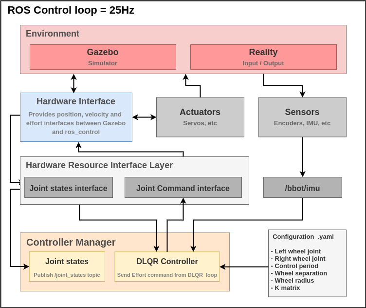 Control DLQR.
We can see in the following videos that the controller performed well in the simulator. It remained stable against external disturbances of up to 800 N and behaved well when receiving linear and angular movement commands.
Next steps
At this stage of the project, we presented the mathematical model of Bbot.
The results for the tests were presented in their respective descriptions. For the next steps, tests with the real robot will be presented, demonstrating the control and its adjustments in practice.
For a more comprehensive approach to the project and how it was done with python control, follow this link.
Author
References
- The original post was published on braziliansinrobotics, which is a project of the Brazilian Institute of Robotics (BIR). The website is no longer available, so I am reposting it here.
This is an automatically translated version of the original post from the site ‘brazilians in robotics’ (no longer available).