
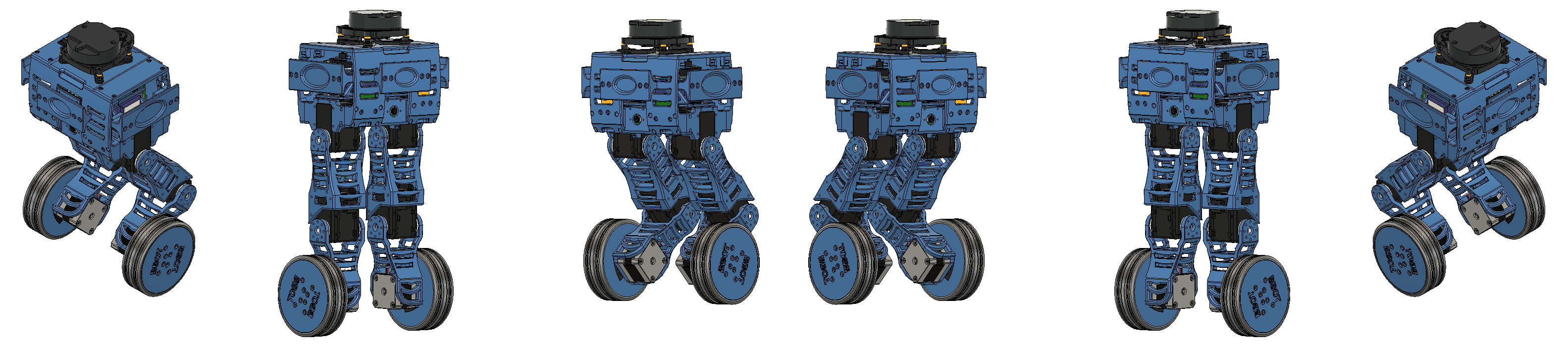
In the last post, we showed how we designed an LQR controller based on a mathematical model of the robot and the results of some simulations we did with this controller. Since then, we have implemented the controller on the real robot and carried out several balancing tests. Today, we’ll talk a bit about this implementation process, the results we achieved, and our perspectives for the project.
Controller implementation on the real robot
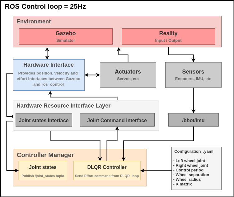
As shown in the last post, we implemented the controller in ROS Noetic using the resources of the ros_control package. The schematic we showed can be seen below and, if you want to know more about it, we recommend checking this link.
 DLQR.
DLQR.
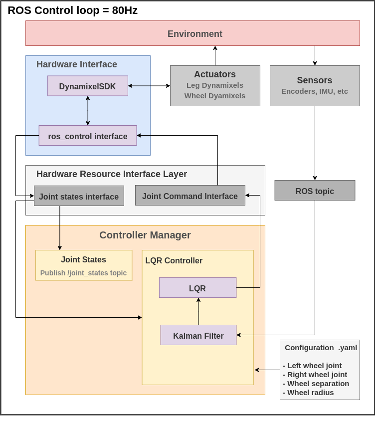
This schematic covers both the real and simulated situations. A more specific model of the real system can be seen below.
 LQR Control.
The main structure remains the same. We created an LQR controller plugin that communicates with the controller_manager from ros_control and updates the control efforts based on the readings from the robot’s joint states and the sensors installed on it—in our case, only the IMU. The robot’s joints are defined and commanded by the hardware_interface, which communicates directly with the robot’s real actuators, handling command writing and reading current states.
The first noticeable change is the control loop frequency, which was set to 80 Hz. This change was necessary to improve control performance. It would be even better if we could increase this frequency further, but this was the fastest we could achieve. This will be discussed in more detail later in the post.
All our actuators are Dynamixel motors, so the hardware_interface uses the DynamixelSDK library to communicate with the motors. The chosen communication channel was a U2D2, a device from ROBOTIS that allows serial communication via USB port. This was the simplest way we found to use the Dynamixels, but it turned out to be quite slow for our application, being one of the main limitations for the control frequency. To reach 80 Hz, we had to isolate the leg motors. At the start of the program, the hardware_interface sends the leg joint angles but no longer reads them. Thus, leg control (yet to be implemented) would be handled in another control loop. By keeping read and write communication only for the two wheel motors, it was possible to reach up to 100 Hz. The reason for lowering it to 80 Hz, besides keeping a margin for communication delays, will be described later.
For good control performance, it’s necessary to have a way to control the motors that is stable, fast-reacting, and as linear as possible. For this, we used the PWM mode of the Dynamixels.
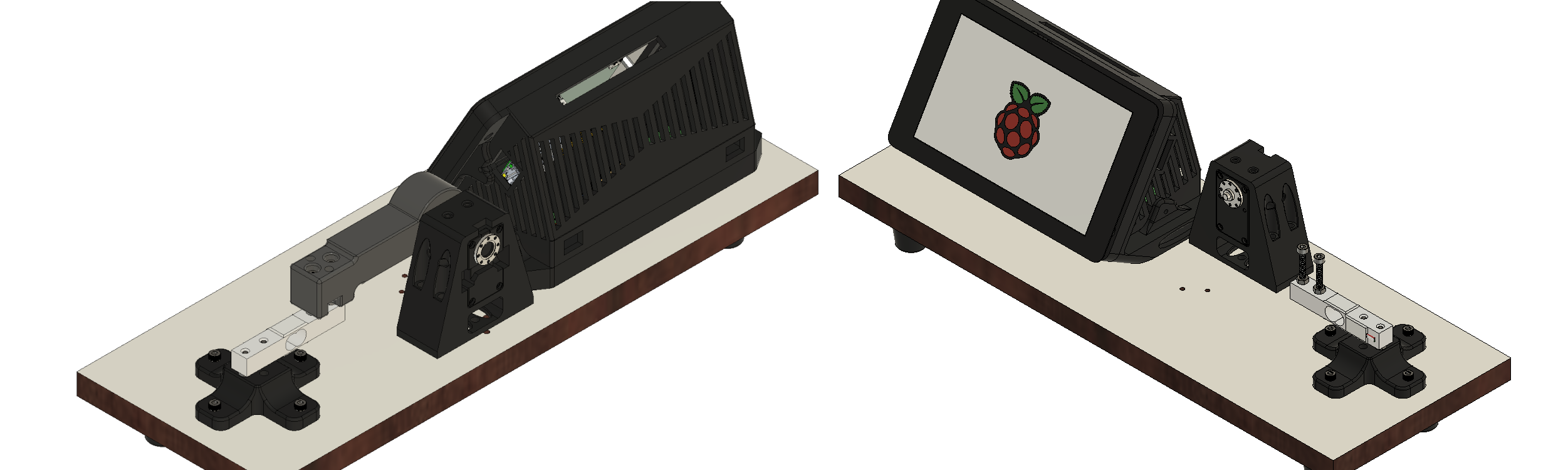
The control algorithm shown in the last post included only an LQR controller, which sends direct torque commands to the robot’s wheels. This was enough for great simulation results, but in practice, it’s necessary to find a relationship between the motor’s PWM signal and the torque it produces. For this, we chose to generate a linear mathematical model of the motors. This model would be the dynamic relationship between the input (PWM signal) and the output (torque), which can be represented by a transfer function. To generate this model, we created a test bench that allows us to measure the torque generated by the motor after sending a PWM signal to it through a load cell. Below is a photo of the test bench. We have a dedicated post about it that we strongly recommend checking at this link.
 Strength Test Bench.
After collecting the data, we used a Python system identification library called SIPPY. It allows us to generate several discrete-time dynamic models, both as transfer functions and in state space, in a simple way. We used the ARX model and generated a first-order transfer function, shown below.
\[\frac{0.00002648}{z-0.8444}\]With the motor model in hand, we included it in the robot’s mathematical model and designed another LQR controller. Now, the system input is no longer the wheel torque but the PWM signal sent to the motor. This step was crucial, because besides having the direct relationship between the PWM signal and the torque (always with some uncertainties, but if the model is good enough, these can be compensated by tuning the controller), we can design an LQR that considers the entire real motor dynamics. Our test bench uses a 20 kg load cell as a sensor, interfacing with a Raspberry via an Hx711 amplifier board. This board operates at a maximum of 80 Hz, which was the frequency we used to collect data and generate the motor model. Since the sampling period of the motor model and the robot model had to be the same, we reduced the control loop from 100 to 80 Hz.
After including the motor dynamics in the robot model, one more adjustment was needed. To use the LQR, it’s necessary to have the current value of all model states. However, it’s not possible to directly measure the wheel torque while the robot is operating. Therefore, we implemented a Kalman filter to estimate the value of these new states (in our case, 2, since we included the dynamics of two first-order models, each with 1 state) based on the readings of the others (linear velocity, pitch angular velocity, yaw angular velocity, and pitch angle).
Tests
After making all the corrections described above, we managed to make the robot balance itself. It can remain stable for several minutes and even recover after small external disturbances. Below you can check out some test videos.
Future Perspectives
Getting the robot to balance itself shows the success of our control system and implementation. But Bbot was designed to be a robot capable of reading TAGs using computer vision and navigating autonomously. For this, its stability needs to be improved. Throughout the project, we received several suggestions from our advisor and colleagues on how to do this. Here are the main ones:
Make the robot’s structure lighter by removing some components, replacing others, and better distributing the weight throughout the structure. The entire casing can be redesigned to use as little material as possible. In addition, we can replace the leg motors with lighter Dynamixel models that are much better suited for this application. Regarding material distribution, the new structure can be designed so that each component is attached respecting the robot’s symmetry. This will prevent the center of mass from shifting relative to the wheel’s contact point with the ground.
Use faster motors on the wheels. Dynamixels are excellent actuators, precise and with a lot of torque, but they are very slow. The model we used was the XM430-W210, which reaches a maximum of 90 rpm. According to our simulations and the size of Bbot’s wheel radius, at least 300 rpm would be needed for a fast enough reaction speed to keep the robot very stable. Also, speeding up communication is essential. To send a PWM signal to the Dynamixel, serial communication via RS-485 protocol is required. It would be faster to send a PWM signal directly to the motor.
Implement the LQR on a microcontroller to make it as fast and precise as possible. The Raspberry Pi was sufficient to support a control loop at 80 Hz with good precision. However, a microcontroller is more suitable for this task, as we can achieve much higher frequencies, increasing the precision of the discretized model, which improves performance.
These were some details of our implementation. We achieved good results, but we know there are many points for improvement in the project. Bbot is an ongoing project and we’ll post updates as they happen.
If you want to learn more about Bbot, be sure to check out our homepage!
Author

References
- The original post was published on braziliansinrobotics, which is a project of the Brazilian Institute of Robotics (BIR). The website is no longer available, so I am reposting it here.
This is an automatically translated version of the original post from the site ‘brazilians in robotics’ (no longer available).