
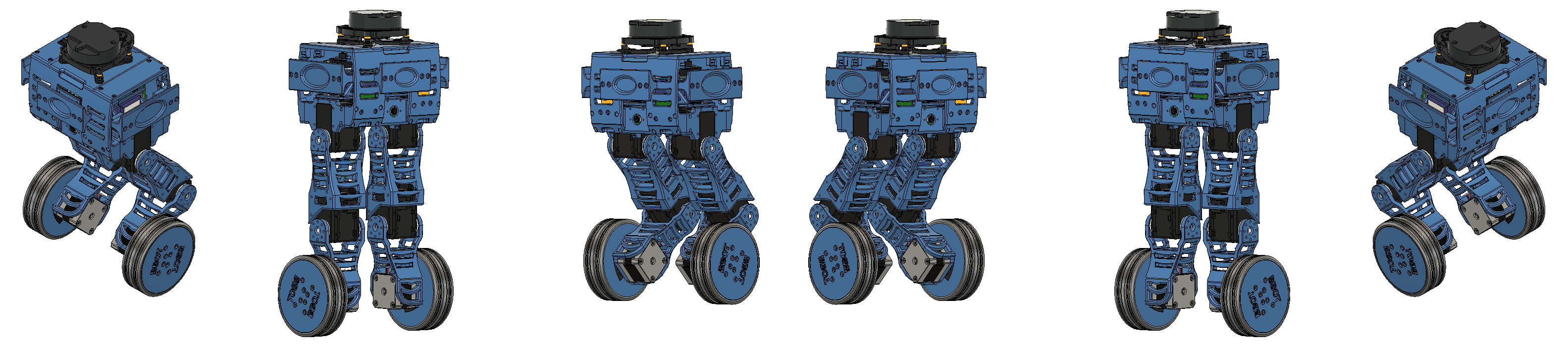
Recently, we showed how we implemented the LQR controller on the real robot and the results we achieved. In that post, which we recommend checking out by clicking this link, we mentioned that Bbot was designed to be a robot capable of reading TAGs via computer vision and autonomously navigating an environment while avoiding obstacles. These features have not yet been implemented on the real prototype, but they are present in the simulation. Today, we want to share a bit about this simulation and show more details about Bbot’s mission.
The Mission
On our official page, we give a brief description of Bbot’s mission. But in case you haven’t checked it out, Bbot is a self-balancing robot that, in addition to balancing and moving on two wheels, must be able to read a TAG (fiducial marker, see image below), which will send the robot a target position to which it must autonomously navigate. To perform navigation, the robot must be able to create a map of its environment and localize itself within it, allowing it to update its position throughout the mission and avoid obstacles while navigating to its goal.
TAG Reading
To read the TAG, we use a ROS package that already has this functionality implemented, developed here in our lab. In addition to containing the entire computer vision algorithm, it already uses the ROS interface, publishing a TF (basically a position relative to a reference frame). By doing this in real time, it is possible to easily use this information in other rosnodes implemented in the system. Knowing the distance from the robot to this TAG, and knowing the TAG’s location in space, we provide the robot with a reference position to which it must autonomously navigate.
 Aruco.
SLAM
To navigate the environment, the robot first needs to know where it is and, if it wants to avoid obstacles, it needs to know where the obstacles are in space. Creating a map of the environment and simultaneously localizing itself within it is a very relevant problem in robotics called SLAM (Simultaneous Localization and Mapping). ROS contains several packages with SLAM algorithms implemented. One of the most used is gmapping, which uses laser sensor readings to identify obstacles in the environment and create a map with information about where the robot can navigate and where obstacles are. In addition, the algorithm also estimates the robot’s position based on the displacement of laser readings collected over a short time interval. This algorithm is quite powerful, and we implemented it on Bbot.
Below you can see one of the images generated from the simulation, where you can compare the simulated environment on the left and the generated map on the right.
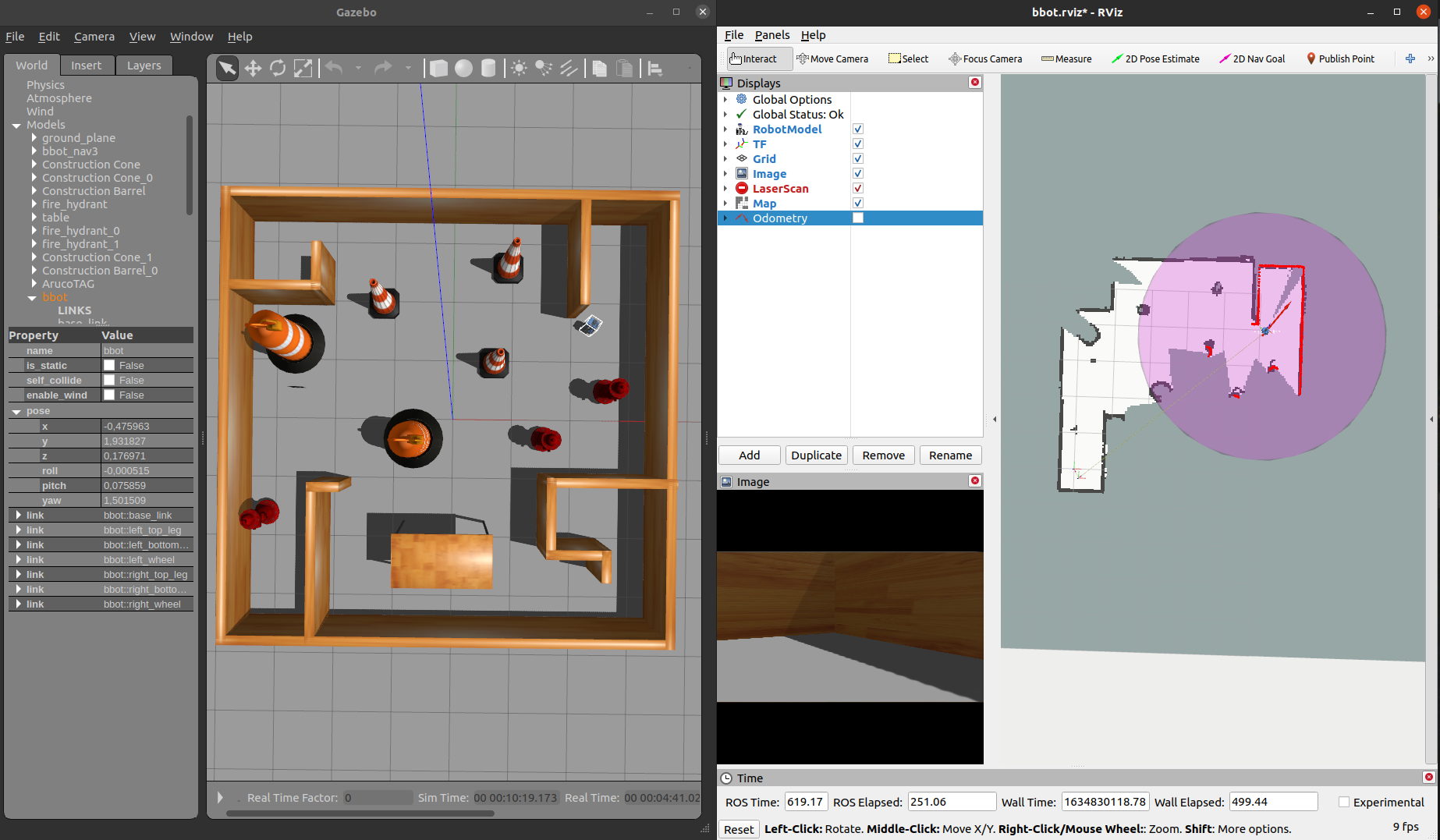 SLAM.
SLAM.
Odometry
Odometry is the use of data to estimate the speed and position of a body in space. It may sound similar to SLAM, but it is broader. Odometry does not assume map creation; it is only concerned with estimating the robot’s displacement in space. For gmapping to recreate the environment map based on laser data, it needs to combine all readings to record points where the laser returned (obstacles) and discard points where there was no light return (free space). For this, it is necessary to know how much the robot has moved so that this “stitching” of laser information (which becomes the map) is done correctly and the environment is recreated as accurately as possible. So, if gmapping already does this, why highlight it again? The point is that, as it is an estimate, errors can occur, and when they accumulate, they hinder navigation by providing the robot with incorrect information about the environment and its location. To solve this, we perform sensor fusion, combining readings from various sources to get the best possible estimate of the information we want. An excellent tool for this is a Kalman Filter (we talked a bit about it in the last post). The ROS package robot_localization implements a variation called the extended Kalman filter, based on the model of a mobile platform. Thus, we can provide it with information from various odometry sources and IMUs to get a better estimate of the robot’s position and speed. Bbot has wheel encoders and an IMU, which are the data sources we provide to robot_localization.
Below is an image showing the robot in the virtual world and the trajectory it followed, represented by the red arrows over time.
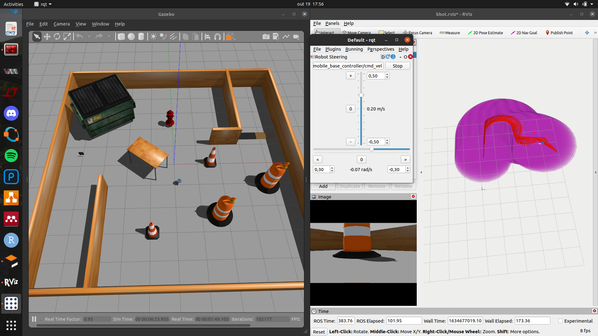 EKF.
EKF.
Move Base Flex + PyTrees
If you’ve ever tried to implement autonomous navigation on a robot using ROS, you’ve probably heard of or used move_base. It is an autonomous navigation interface that, based on a map of the environment, the robot’s current position, and a target position, can calculate a trajectory to this point, avoiding obstacles, and, through a controller, send velocity commands to the robot to guide it to its goal. move_base is another excellent tool provided in ROS, but it has some shortcomings, especially when the algorithm fails to guide the robot. Therefore, another navigation interface was created, very similar, with the same base algorithms but more flexible, allowing developers to dictate the robot’s behavior in case of planning or control failures, making the system much more robust. This is move_base_flex. And to manage all these tasks—planning the trajectory, guiding the robot along the path, identifying errors, and correcting them—we use a very versatile control architecture called a Behavior Tree. The py_trees package implements this architecture in Python, and through py_trees_ros, we can use some ROS functionalities in our Behavior Tree.
Also, through the Behavior Tree, we can use the TAG detection data (the robot’s position relative to it) to set a goal for the robot. Because detection errors can occur and the TAG position can be updated, we must also update the target position. This is another functionality implemented in Bbot via the Behavior Tree.
If you have never heard of any of these packages or concepts before and want to learn more, I suggest checking the links below:
Simulation
After implementing odometry, SLAM, TAG detection, and autonomous navigation managed via a Behavior Tree, we proceeded with the robot simulation. Below, you can see some gifs and videos we made, demonstrating Bbot’s operation.
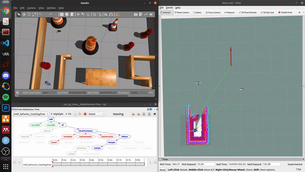 Navigation.
Unlike the image shown in the gmapping section, in these, the obstacles have a colored envelope. This is a region created by the ROS package costmap2d, which move_base_flex uses to enlarge the size of obstacles so that the trajectory controller tries to avoid these regions.
Although we talked a bit about the improvements we intend to implement in the real Bbot model in the last post, so it can accomplish its final mission, we didn’t talk much about the mission itself. I hope this post has clarified more about our plans for this robot and the path we intend to follow. Bbot is a work in progress, and we will post updates as soon as we have more news.
Author

References
- The original post was published on braziliansinrobotics, which is a project of the Brazilian Institute of Robotics (BIR). The website is no longer available, so I am reposting it here.
This is an automatically translated version of the original post from the site ‘brazilians in robotics’ (no longer available).